🎯 06. デジタル H∞ 制御 / Digital H∞ Control
ℹ️ 数式が正しく表示されない場合はGitHub版をご確認ください
If equations do not render properly, see the GitHub version
📖 概要 / Overview
デジタル H∞ 制御は、ロバスト制御の一種であり、外乱やモデル誤差に対して安定性と性能を保証する制御器を、離散時間系で設計する手法です。
Digital H∞ control is a robust control approach implemented in discrete time, designed to ensure stability and performance against disturbances and model uncertainties.
本教材では、連続時間 H∞ 設計 → 離散化 → デジタル実装 → 周波数応答評価 の流れを示します。
This material covers the flow from continuous-time H∞ design → discretization → digital implementation → frequency response evaluation.
🎯 学習目標 / Learning Goals
- H∞ 制御の基本構造を理解する
Understand the basic structure of H∞ control - 連続時間 H∞ 制御器を MATLAB で設計できる
Design continuous-time H∞ controllers in MATLAB - 離散化方法(双一次変換など)を理解する
Understand discretization methods such as bilinear transform - Simulink モデルで動作を検証できる
Validate the controller behavior using Simulink
📐 制御問題の定義 / Problem Formulation
感度関数と補償関数 / Sensitivity and Complementary Sensitivity
\[S(s) = \frac{1}{1 + G(s)K(s)}, \quad T(s) = 1 - S(s)\]- $S(s)$:外乱抑制性能(低周波域で小さく)
$S(s)$: Disturbance rejection (small at low frequencies) - $T(s)$:ノイズ抑制性能(高周波域で小さく)
$T(s)$: Noise attenuation (small at high frequencies)
H∞ 最適化条件 / H∞ Optimization Objective
\[\lVert T_{zw}(s) \rVert_\infty < \gamma\]- $T_{zw}(s)$:外乱 $w$ から性能出力 $z$ への伝達関数
$T_{zw}(s)$: Transfer function from disturbance $w$ to performance output $z$ - $\lVert \cdot \rVert_\infty$ :全周波数帯域での最大ゲイン(無限ノルム)
$\lVert \cdot \rVert_\infty$ : Maximum gain over all frequencies (infinity norm)
🛠️ MATLABによる設計例 / MATLAB Design Example
% 状態空間モデル例 / Example state-space model
A = [...]; B = [...]; C = [...]; D = zeros(size(C,1), size(B,2));
P = ss(A,B,C,D);

% 重み付け関数(性能W1, 制御W2) / Weighting functions (Performance W1, Control W2)
s = tf('s');
W1 = (s/10 + 1)/(s/100 + 1);   % 感度関数重み / Sensitivity weight
W2 = (s/100 + 1)/(s/1000 + 1); % 補償関数重み / Control effort weight
Paug = augw(P, W1, W2);

% H∞制御器設計 / H∞ controller design
nmeas = 1; ncon = 1;
[K,CL,gamma] = hinfsyn(Paug, nmeas, ncon);

% 性能確認 / Performance check
sigma(CL); grid on
disp("H∞ gamma = " + gamma);
🔄 離散化 / Discretization
サンプリング周期の選定 / Choosing the sampling period
- 応答帯域の 1/10 程度を目安に設定
Typically set to about 1/10 of the response bandwidth - 例:帯域が 100 Hz → $T_s \approx 1 \ \mathrm{ms}$
Example: bandwidth = 100 Hz → $T_s \approx 1 \ \mathrm{ms}$
双一次変換(Tustin法)による離散化 / Bilinear transform (Tustin method)
Ts = 0.001;                 % 1 ms サンプリング / Sampling
Kd = c2d(K, Ts, 'tustin');  % デジタル制御器 / Digital controller
🧪 Simulinkによる検証 / Validation with Simulink
- Simulinkモデル
digital_hinf_simulink.slxで閉ループを構成
Build a closed-loop system in Simulink usingdigital_hinf_simulink.slx - 外乱入力、測定ノイズを加えて $S(z)$、$T(z)$ の挙動を確認
Add disturbance input and measurement noise to observe $S(z)$ and $T(z)$ behavior - ステップ応答と周波数応答を比較
Compare step response and frequency response
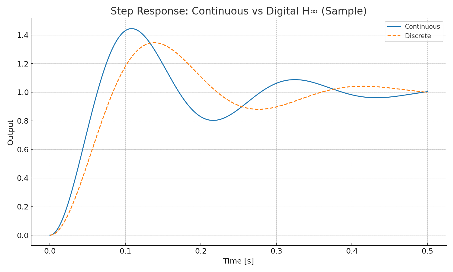
図1 / Fig.1 — ステップ応答(連続 vs 離散H∞)
連続設計と離散実装の応答を比較。離散側はわずかに帯域が低く、減衰が大きい。
Step responses of continuous design and digital implementation. The digital one shows slightly lower bandwidth and higher damping.
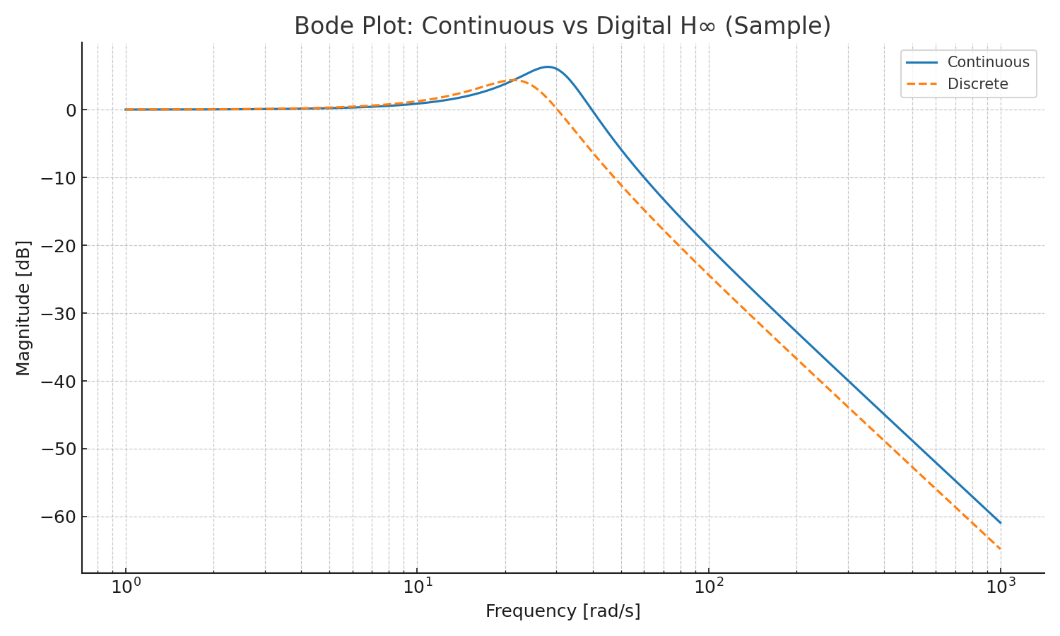
図2 / Fig.2 — ボード線図(連続 vs 離散H∞)
中高周波でのゲイン差を可視化し、離散化の影響を確認。
Bode magnitude comparison highlighting mid–high frequency differences due to discretization.
📊 ロバスト性評価 / Robustness Metrics
| 指標 / Metric | 説明 / Description | 目安 / Guideline | 評価 / Rating |
|---|---|---|---|
| ゲイン余裕 GM | 増幅許容量 / Gain tolerance | > 6 dB | ○ |
| 位相余裕 PM | 遅延許容量 / Phase tolerance | > 30° | ○ |
| $\lVert S \rVert_\infty$ | 感度関数の無限ノルム / Infinity norm of sensitivity | < 2.0 | ◎ |
Note: $\lVert S \rVert_\infty$ が小さいほど外乱に強い。2.0 は約 6 dB に相当。
Note: The smaller $\lVert S \rVert_\infty$, the stronger the disturbance rejection. 2.0 ≈ 6 dB.
💡 実装のヒント / Implementation Notes
- 固定小数点化時の量子化誤差対策
Mitigation of quantization errors during fixed-point conversion - 演算遅延の位相余裕への影響評価
Evaluate the impact of computational delay on phase margin - Simulink Coder による C コード生成 → FPGA実装(
SoC_DesignKit_by_ChatGPT/c_to_hdl/)
Generate C code using Simulink Coder → FPGA implementation (SoC_DesignKit_by_ChatGPT/c_to_hdl/)
📚 参考文献 / References
- Zhou & Doyle, Essentials of Robust Control
- Skogestad & Postlethwaite, Multivariable Feedback Control
- MATLAB Robust Control Toolbox Documentation
⬅️ 前節 / Previous: 05. FFTによる信号分析と雑音除去 / FFT-based Signal Analysis and Noise Removal
🏠 第4章トップ / Chapter 4 Top: デジタル制御と信号処理 / Digital Control and Signal Processing
➡️ 次章 / Next Chapter: Part 05: 実装・応用演習 / Implementation & Application Practice