🎞️ AITL Animation Demos
This page provides quick access to experimental animation demos related to AITL (Architecture for Integrated Technology Logic) concepts.
Each demo is self-contained and can be viewed directly in the browser without additional setup. 🚀
🔗 Links
| Language | GitHub Pages 🌐 | GitHub 💻 |
|---|---|---|
| 🇺🇸 English |
🎨 CSS-only Demos
Pure CSS animations focusing on conceptual clarity and minimal dependencies.
-
🪐 Orbit Demo (FSM concept)
Conceptual orbit-style animation using pure CSS, representing FSM state circulation.
👉 Open demo -
✨ Fade-in Demo
Simple fade-in animation for step-by-step concept introduction and explanation flow.
👉 Open demo -
💓 Pulse Demo (Attention highlight)
Pulse animation to subtly emphasize important elements without distraction.
👉 Open demo -
🧱 Layer Stack Demo (AITL layers)
Stacked animation visualizing the PID → FSM → LLM layered architecture of AITL.
👉 Open demo
🧩 JS + SVG Demos
Interactive demos combining JavaScript logic with SVG-based visualization.
-
🔄 AITL Control Flow Demo
Demonstrates the full AITL loop:
PID response → disturbance → FSM detection → LLM gain re-tuning → target re-tracking
👉 Open demo -
🧪 PZT Perovskite Unit Cell Demo (JS + SVG)
Single perovskite unit cell visualization focusing on B-site (Zr/Ti) off-centering
inside a rigid O₆ octahedron, with subtle z-direction lattice relaxation.
👉 Open demo
🖌️ Canvas Demos
Physics-inspired visualizations using the HTML5 Canvas API.
- 💧 Inkjet Droplet Formation Demo (Canvas)
Particle-based visualization of:- inkjet droplet ejection
- main droplet formation
- satellite droplets
- substrate impact
Drive voltage V and current I are shown as conceptual parameters
to illustrate qualitative behavior changes.⚠️ This demo is intended for intuitive understanding only
and is not a physical simulation or CFD analysis.
🧠 These demos are designed as visual thinking tools to support AITL education, explanation, and rapid conceptual prototyping.
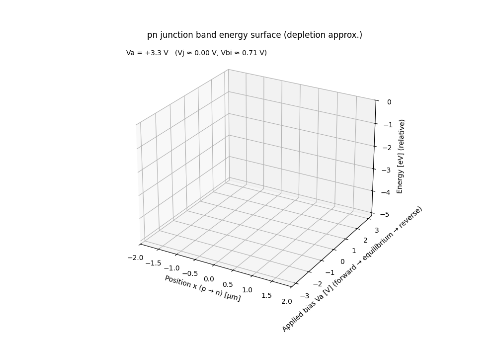
⚡ PN Junction Band Energy Surface (Bias Sweep)
This animation visualizes the energy-band surface of a pn junction under a continuous bias sweep from forward → equilibrium → reverse.
- 📏 x-axis: Spatial position across the junction
(p-type → n-type) - 🔌 y-axis: Applied junction bias $V_a$
(forward → equilibrium → reverse) - 📈 z-axis: Energy (relative, eV)
The band surface is constructed using a depletion approximation to emphasize the geometric structure of the electrostatic potential rather than carrier transport details.
🧠 Physical interpretation
This 3D representation unifies what are traditionally shown as separate 2D band diagrams:
- ➕ Forward bias: potential barrier collapses
- ⚖️ Equilibrium: built-in potential forms a stable barrier
- ➖ Reverse bias: depletion region widens and deepens
Any conventional textbook pn-junction band diagram corresponds to a 2D slice of this surface at a fixed bias.
Likewise, fixing position and sweeping bias reveals how the electrostatic barrier evolves continuously—something difficult to grasp from static figures alone.
🧩 Modeling assumptions
- Abrupt pn junction
- Uniform doping on both sides
- Depletion approximation
- Energy plotted as
$E_c(x) \propto -\phi(x)$ (relative scale)
Carrier injection, recombination, and quasi-Fermi level splitting are intentionally omitted to keep the visualization focused on electrostatic structure.
This animation serves as the electrostatic foundation for the MOS and NMOS visualizations that follow.
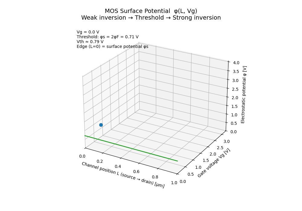
🟦 MOS Surface Potential
(Weak Inversion → Threshold → Strong Inversion)
This animation visualizes the MOS surface potential $(\phi(L, V_g))$ as a continuous function of channel position and gate voltage, explicitly connecting:
weak inversion → threshold → strong inversion
📐 Axes definition
- 📏 x-axis: Channel position $(L)$
(source → drain) - 🔌 y-axis: Gate voltage $(V_g)$
- 📊 z-axis: Electrostatic potential $(\phi)$
The potential surface is constructed using a minimal educational model to emphasize physical intuition rather than compact-model accuracy.
🔍 Physical meaning
The total potential is decomposed as:
- a linear source–drain component along the channel, and
- a gate-controlled surface modulation that decays away from the source.
The highlighted edge at $(L = 0)$ ** represents the
**surface potential $(\phi_s(V_g))$.
🎯 Threshold definition
The threshold condition is defined geometrically as:
\[\phi_s = 2\phi_F\]- 🌱 Weak inversion: $(\phi_s < 2\phi_F)$
- 🚩 Threshold (V_th): $(\phi_s = 2\phi_F)$
- 🌊 Strong inversion: $(\phi_s \gtrsim 2\phi_F)$
This makes the threshold voltage not an abstract parameter, but a visible point on the surface, determined by the internal electrostatic state.
✨ Why this representation matters
Traditional MOS explanations separate:
- surface potential,
- threshold voltage,
- and drain current equations.
This animation unifies them by showing that:
Threshold is simply the gate voltage at which the surface potential
reaches the inversion condition.
The transition from weak to strong inversion is therefore a continuous electrostatic process, not a sudden event.
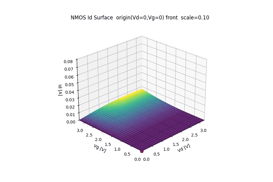
🔺 NMOS $I_d$ Surface
($V_g$ – $V_d$ – $I_d$ Characteristics)
This animation visualizes the NMOS drain current surface $I_d(V_g, V_d)$ under a 3.3 V CMOS operating range.
- 🔌 x-axis: Drain voltage $V_d$ (0 → 3.3 V)
- 🎛️ y-axis: Gate voltage $V_g$ (0 → 3.3 V)
- 📈 z-axis: Drain current $I_d$
The origin $(V_d, V_g) = (0, 0)$ is intentionally placed at the front corner to preserve physical intuition:
- zero gate bias and zero drain bias → zero current
- increasing $V_g$ → enhanced channel inversion
- increasing $V_d$ → transition from linear region to saturation
🧮 Modeling assumptions
The surface is generated using a simplified long-channel NMOS model:
- Threshold voltage: $V_\mathrm{th}$
-
Square-law behavior:
- Linear region:
- Saturation region:
Channel-length modulation and short-channel effects are intentionally omitted to keep the geometric structure of the surface clear.
🔄 Animation behavior
- The surface is periodically scaled (0 → max → 0) to emphasize the topology of the $I_d$ surface without changing the bias axes.
- Viewpoint and axis directions are fixed so that:
- $(V_d, V_g) = (0,0)$ remains at the front,
- higher voltages extend toward the back,
- comparison with electrostatic potential animations is intuitive.
This representation is intended for educational and architectural visualization, not compact model accuracy.
🎛️ PID Control: Visual Intuition by Step Response
This section introduces PID control using minimal step-response animations.
The goal is not mathematical completeness, but instant physical intuition.
We consider a simple control loop where:
- 🔌 Control input: voltage $V$
- 📈 System output: current $I$
- 🎯 Reference: $I_{\mathrm{ref}}$
The controller computes the control voltage $V(t)$ from the current error:
\[e(t) = I_{\mathrm{ref}} - I(t)\]🟦 P Control — Proportional Action
P control reacts only to the instantaneous error.
\[V(t) = K_p \, e(t)\]- ❗ Large error → large control effort
- 🤏 Small error → weak control effort
As shown below:
- 🐢 Low $K_p$: slow response
- ⚡ High $K_p$: fast but overshoots and oscillates
- ❌ Steady-state error always remains
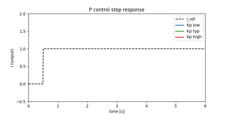
🧠 Key intuition
P control is fast, but it stops acting once the error becomes small.
Precision is impossible with P alone.
🟩 PI Control — Eliminating Steady-State Error
I control accumulates error over time.
\[V(t) = K_p e(t) + K_i \int e(t)\,dt\]To highlight its role, a disturbance is applied during operation.
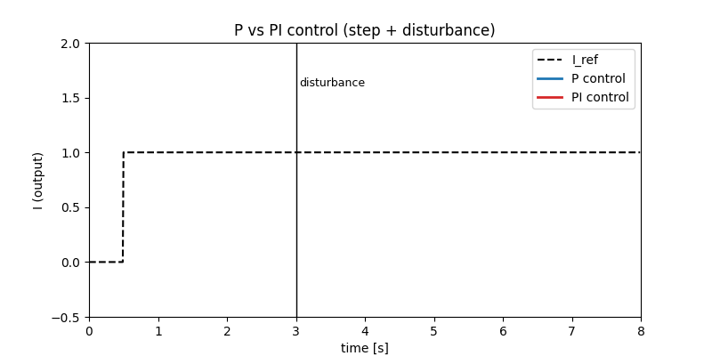
📌 Observation:
- P control leaves a permanent offset after disturbance
- PI control slowly but surely restores the target current
🧠 Key intuition
I control provides persistence.
As long as error exists, it keeps pushing.
🟥 PID Control — Damping Oscillation
D control reacts to the rate of change of the output.
\[V(t) = K_p e(t) + K_i \int e(t)\,dt - K_d \frac{dI}{dt}\]It acts as a dynamic brake, suppressing overshoot and oscillation.
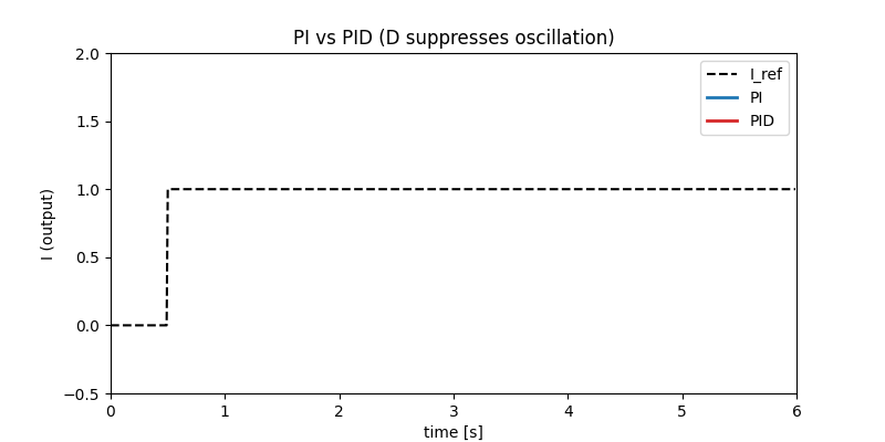
🔍 Comparison:
- PI: reaches the target but oscillates
- PID: reaches the target smoothly and quickly
🧠 Key intuition
D control anticipates motion and applies braking force.
🧩 Summary: Physical Meaning of PID
| Term | Looks at | Physical role |
|---|---|---|
| P | Error | Immediate force |
| I | Accumulated error | Bias removal |
| D | Rate of change | Damping / braking |
🧍 PID control mirrors human motion control:
- 👉 Push toward the target (P),
- 🔁 Keep pushing if still off (I),
- ✋ Brake before overshooting (D).
These animations are designed for architectural understanding and control intuition, rather than parameter tuning or model accuracy.
🧠 FSM (Finite State Machine): Event-Driven Control Logic
PID control explains continuous-time behavior
(voltage–current dynamics and transient response).
FSM governs discrete decision logic:
Is this action allowed now?
Should the control mode change?
- PID answers “how strongly to act”
- FSM answers “whether the action is permitted”
🔁 FSM Visualizer — Discrete State Transition Mechanism
Below is an embedded FSM animation.
The animation runs directly on this page.
👀 How to read this animation
- 🔵 The system is always in exactly one state
- 📥 Events arrive from outside
- 🔀 A state transition occurs only if:
- the event is defined for the current state, and
- the transition condition is satisfied
- 🚫 Invalid events are rejected and cause no state change
| Visual element | Meaning |
|---|---|
| ⚪ Circle | State |
| 🟡 Highlighted circle | Active state |
| ➡️ Arrow | Allowed transition |
| ✨ Moving particle | Incoming event |
| ❌ Disappearing particle | Invalid / rejected event |
This demonstrates the core FSM rule:
State transitions are discrete, conditional, and event-triggered.
🧩 Why FSM Is Required Beyond PID
PID:
- 🔄 Always reacts
- 📤 Always outputs a control signal
- ❓ Cannot decide whether it should act
FSM:
- 🗂 Separates modes (IDLE / RUN / ERROR / RECOVERY)
- 🛡 Enforces safety and permissions
- 📐 Guarantees deterministic behavior
PID controls motion.
FSM controls permission.
🏗 Position of FSM in AITL Architecture
- ⚙️ PID — inner continuous-time loop
- 🧠 FSM — supervisory discrete logic
- 🌐 LLM — outer adaptive layer (rewrites rules or gains)
The embedded FSM animation above is the bridge between time-domain PID intuition and full AITL control flow.
📝 Notes
- 🧪 These demos are experimental and may change without notice.
- 🧭 Not all demos are intended for adoption into the main portal.
- 🗺 This page serves as a navigation hub only.
👤 Author
| 📌 Item | Details |
|---|---|
| Name | Shinichi Samizo |
| Expertise | Semiconductor devices (logic, memory, high-voltage mixed-signal) Thin-film piezo actuators for inkjet systems Printhead productization, BOM management, ISO training |
| GitHub |
📄 License
| 📌 Item | License | Description |
|---|---|---|
| Source Code | MIT License | Free to use, modify, and redistribute |
| Text Materials | CC BY 4.0 or CC BY-SA 4.0 | Attribution required; share-alike applies for BY-SA |
| Figures & Diagrams | CC BY-NC 4.0 | Non-commercial use only |
| External References | Follow the original license | Cite the original source properly |
💬 Feedback
Suggestions, improvements, and discussions are welcome via GitHub Discussions.